如何开发适用于MNIST手写数字分类的CNN
MNIST手写数字分类问题是用于计算机视觉和深度学习的标准数据集。
虽然数据集得到了有效的解决,但它可以作为学习和实践如何从头开始开发、评估和使用卷积深度学习神经网络进行图像分类的基础。这包括如何开发健壮的测试工具来评估模型的性能,如何探索对模型的改进,以及如何保存模型并在以后加载它以对新数据进行预测。
在本教程中,你将了解如何从头开始开发用于手写数字分类的卷积神经网络。
完成本教程后,你将了解:
- 如何开发测试工具来开发模型的健壮评估,并为分类任务建立性能基线。
- 如何探索基线模型的扩展以提高学习和建模能力。
- 如何开发最终的模型,评估最终模型的性能,并使用它对新图像进行预测。
我们开始吧。
教程概述
本教程分为五个部分;它们是:
- MNIST手写数字分类数据集。
- 模型评价方法论。
- 如何开发基线模型。
- 如何开发一种改进的模型。
- 如何最终确定模型并做出预测。
开发环境
本教程假设你使用的是在带有Python 3的TensorFlow之上运行的独立Keras。如果你需要有关设置开发环境的帮助,请参阅此教程:
MNIST手写数字分类数据集。
MNIST数据集是修改后的国家标准与技术研究所数据集的首字母缩写。
它是一个包含60,000个小正方形28×28像素灰度图像的数据集,这些图像是0到9之间的手写单位数。
任务是将给定的手写数字图像分类到10个类别中的一个,这些类别代表从0到9的整数值(包括0到9)。
它是一个广泛使用和深入理解的数据集,并且在很大程度上是“已解决的”。性能最好的模型是深度学习卷积神经网络,它们的分类准确率在99%以上,在坚持测试数据集上的错误率在0.4%到0.2%之间。
下面的示例使用Keras API加载MNIST数据集,并创建训练数据集中前九个图像的绘图。
# example of loading the mnist dataset
from keras.datasets import mnist
from matplotlib import pyplot
# load dataset
(trainX, trainy), (testX, testy) = mnist.load_data()
# summarize loaded dataset
print('Train: X=%s, y=%s' % (trainX.shape, trainy.shape))
print('Test: X=%s, y=%s' % (testX.shape, testy.shape))
# plot first few images
for i in range(9):
	# define subplot
	pyplot.subplot(330 + 1 + i)
	# plot raw pixel data
	pyplot.imshow(trainX[i], cmap=pyplot.get_cmap('gray'))
# show the figure
pyplot.show()
运行该示例将加载MNIST训练和测试数据集,并打印它们的形状。
我们可以看到,在训练数据集中有60,000个示例,在测试数据集中有10,000个示例,并且图像确实是28×28像素的正方形。
Train: X=(60000, 28, 28), y=(60000,)Test: X=(10000, 28, 28), y=(10000,)
还创建数据集中前九个图像的曲线图,显示待分类图像的自然手写性质。
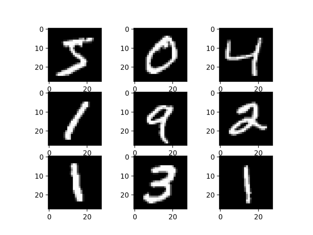 绘制MNIST数据集中的图像子集
模型评价方法论
虽然MNIST数据集得到了有效的解决,但对于开发和实践使用卷积神经网络解决图像分类任务的方法来说,它可以是一个有用的起点。
我们可以从头开始开发一个新的模型,而不是查看关于数据集上性能良好的模型的文献。
数据集已经有了我们可以使用的定义良好的训练和测试数据集。
为了估计模型在给定训练运行时的性能,我们可以进一步将训练集拆分成训练和验证数据集。然后,可以绘制每次运行的训练和验证数据集上的性能,以提供学习曲线,并深入了解模型学习问题的情况。
Keras API通过在训练模型时将“validation_data”参数指定给model.fit()函数来支持这一点,该函数将返回一个对象,该对象描述所选损失的模型性能和每个训练时期的指标。
# record model performance on a validation dataset during training
history = model.fit(..., validation_data=(valX, valY))
为了在总体上估计模型在问题上的性能,我们可以使用k次交叉验证,也许是5次交叉验证。这将给出关于训练和测试数据集中的差异以及关于学习算法的随机性质的模型方差的一些解释。在给定标准偏差的情况下,可以将模型的性能视为k倍上的平均性能,如果需要,可以使用该平均性能来估计置信区间。
我们可以使用scikit-learn API中的KFold类来实现给定神经网络模型的k重交叉验证评估。虽然我们可以选择一种灵活的方法,其中KFold类仅用于指定用于每个spit的行索引,但有很多方法可以实现这一点。
# example of k-fold cv for a neural net
data = ...
# prepare cross validation
kfold = KFold(5, shuffle=True, random_state=1)
# enumerate splits
for train_ix, test_ix in kfold.split(data):
        model = ...
	...
我们将保留实际的测试数据集,并将其用作最终模型的评估。
如何开发基线模型
第一步是开发基线模型。
这是至关重要的,因为它既涉及为测试工具开发基础设施,以便我们设计的任何模型都可以在数据集上进行评估,又建立了关于问题的模型性能的基线,所有改进都可以根据该基线进行比较。
测试工具的设计是模块化的,我们可以为每个部件开发单独的功能。如果我们愿意,这允许修改或互换测试工具的给定方面,与其他方面分开。
我们可以用五个关键要素来开发这个测试工具。它们是数据集的加载、数据集的准备、模型的定义、模型的评估和结果的呈现。
加载数据集
我们知道一些关于数据集的事情。
例如,我们知道图像都是预先对齐的(例如,每个图像只包含一个手绘数字),图像都具有相同的28×28像素的正方形大小,并且图像都是灰度的。
因此,我们可以加载图像并重塑数据数组,使其具有单一颜色通道。
# load dataset
(trainX, trainY), (testX, testY) = mnist.load_data()
# reshape dataset to have a single channel
trainX = trainX.reshape((trainX.shape[0], 28, 28, 1))
testX = testX.reshape((testX.shape[0], 28, 28, 1))
我们还知道有10个类,并且类被表示为唯一的整数。
因此,我们可以对每个样本的类元素使用1热编码,将整数转换为10个元素的二进制向量,类值的索引为1,所有其他类的值为0。我们可以使用to_categorical()实用函数来实现这一点。
# one hot encode target values
trainY = to_categorical(trainY)
testY = to_categorical(testY)
load_dataset()函数实现这些行为,并可用于加载数据集。
# load train and test dataset
def load_dataset():
	# load dataset
	(trainX, trainY), (testX, testY) = mnist.load_data()
	# reshape dataset to have a single channel
	trainX = trainX.reshape((trainX.shape[0], 28, 28, 1))
	testX = testX.reshape((testX.shape[0], 28, 28, 1))
	# one hot encode target values
	trainY = to_categorical(trainY)
	testY = to_categorical(testY)
	return trainX, trainY, testX, testY
准备像素数据
我们知道数据集中每个图像的像素值都是黑白或0到255之间的无符号整数。
我们不知道缩放建模像素值的最佳方式,但我们知道需要一些缩放。
一个很好的起点是规格化灰度图像的像素值,例如将它们重新缩放到范围[0,1]。这包括首先将数据类型从无符号整数转换为浮点数,然后将像素值除以最大值。
# convert from integers to floats
train_norm = train.astype('float32')
test_norm = test.astype('float32')
# normalize to range 0-1
train_norm = train_norm / 255.0
test_norm = test_norm / 255.0
下面的prep_pixels()函数实现了这些行为,并为需要缩放的训练和测试数据集提供了像素值。
# scale pixels
def prep_pixels(train, test):
	# convert from integers to floats
	train_norm = train.astype('float32')
	test_norm = test.astype('float32')
	# normalize to range 0-1
	train_norm = train_norm / 255.0
	test_norm = test_norm / 255.0
	# return normalized images
	return train_norm, test_norm
在任何建模之前,必须调用此函数来准备像素值。
定义模型
接下来,我们需要为该问题定义一个基线卷积神经网络模型。
该模型主要包括两个方面:特征提取前端(由卷积和池层组成)和分类器后端(进行预测)。
对于卷积前端,我们可以从具有小滤波器大小(3,3)和适度数量的滤波器(32)的单个卷积层开始,然后是最大汇聚层。然后,过滤器地图可以被展平以向分类器提供特征。
假设该问题是一个多类别分类任务,我们知道我们将需要一个具有10个节点的输出层,以便预测属于这10个类别中每一个类别的图像的概率分布。这还需要使用softmax激活功能。在特征提取器和输出层之间,我们可以添加一个致密层来解释特征,在本例中有100个节点。
所有层都将使用ReLU激活功能和权重初始化方案,这两者都是最佳实践。
我们将对随机梯度下降优化器使用保守配置,学习率为0.01,动量为0.9。分类交叉熵损失函数将被优化,适合于多类分类,我们将监控分类精度度量,这是合适的,因为我们在10个类中的每一个中都有相同数量的示例。
下面的 define_model()函数将定义并返回此模型。
# define cnn model
def define_model():
	model = Sequential()
	model.add(Conv2D(32, (3, 3), activation='relu', kernel_initializer='he_uniform', input_shape=(28, 28, 1)))
	model.add(MaxPooling2D((2, 2)))
	model.add(Flatten())
	model.add(Dense(100, activation='relu', kernel_initializer='he_uniform'))
	model.add(Dense(10, activation='softmax'))
	# compile model
	opt = SGD(lr=0.01, momentum=0.9)
	model.compile(optimizer=opt, loss='categorical_crossentropy', metrics=['accuracy'])
	return model
评估模型
在定义了模型之后,我们需要对其进行评估。
该模型将使用五重交叉验证进行评估。选择k=5的值是为了提供重复评估的基线,并且不会太大以至于需要很长的运行时间。每个测试集将是训练数据集的20%,或约12,000个示例,接近此问题的实际测试集的大小。
训练数据集在拆分之前被打乱,每次都会执行样本打乱,这样我们评估的任何模型在每个文件夹中都将具有相同的训练和测试数据集,从而在模型之间提供了相似的比较。
我们将为10个训练周期训练基线模型,默认批次大小为32个示例。每个折叠的测试集将用于在训练运行的每个时期评估模型,以便我们可以在稍后创建学习曲线,以及在运行结束时,以便我们可以估计模型的性能。因此,我们将跟踪每次运行产生的历史记录,以及折叠的分类准确性。
下面的evaluate_model()函数实现了这些行为,它将训练数据集作为参数,并返回稍后可以总结的准确度分数和训练历史列表。
# evaluate a model using k-fold cross-validation
def evaluate_model(dataX, dataY, n_folds=5):
	scores, histories = list(), list()
	# prepare cross validation
	kfold = KFold(n_folds, shuffle=True, random_state=1)
	# enumerate splits
	for train_ix, test_ix in kfold.split(dataX):
		# define model
		model = define_model()
		# select rows for train and test
		trainX, trainY, testX, testY = dataX[train_ix], dataY[train_ix], dataX[test_ix], dataY[test_ix]
		# fit model
		history = model.fit(trainX, trainY, epochs=10, batch_size=32, validation_data=(testX, testY), verbose=0)
		# evaluate model
		_, acc = model.evaluate(testX, testY, verbose=0)
		print('> %.3f' % (acc * 100.0))
		# stores scores
		scores.append(acc)
		histories.append(history)
	return scores, histories
目前的结果
一旦对模型进行了评估,我们就可以展示结果了。
提出了两个关键问题:模型在训练过程中学习行为的诊断和模型性能的估计。这些可以使用单独的函数来实现。
首先,诊断涉及在k折交叉验证的每一次折叠期间创建显示列车和测试集上的模型性能的线状图。这些曲线图对于了解模型是否过度拟合、不足拟合或是否与数据集很好拟合很有价值。
我们将创建一个包含两个子图的单个图形,一个用于损失,另一个用于精度。蓝线将指示训练数据集的模型性能,橙线将指示坚持测试数据集的性能。下面的summarize_diagnostics()函数根据收集的训练历史创建并显示此图。
# plot diagnostic learning curves
def summarize_diagnostics(histories):
	for i in range(len(histories)):
		# plot loss
		pyplot.subplot(2, 1, 1)
		pyplot.title('Cross Entropy Loss')
		pyplot.plot(histories[i].history['loss'], color='blue', label='train')
		pyplot.plot(histories[i].history['val_loss'], color='orange', label='test')
		# plot accuracy
		pyplot.subplot(2, 1, 2)
		pyplot.title('Classification Accuracy')
		pyplot.plot(histories[i].history['accuracy'], color='blue', label='train')
		pyplot.plot(histories[i].history['val_accuracy'], color='orange', label='test')
	pyplot.show()
接下来,可以通过计算平均值和标准差来汇总在每个折叠过程中收集的分类准确率分数。这提供了在该数据集上训练的模型的平均预期性能的估计,以及均值中的平均方差的估计。我们还将通过创建和展示盒子和胡须情节来总结分数的分布。
下面的summarize_performance()函数为模型评估期间收集的给定分数列表实现这一点。
# summarize model performance
def summarize_performance(scores):
	# print summary
	print('Accuracy: mean=%.3f std=%.3f, n=%d' % (mean(scores)*100, std(scores)*100, len(scores)))
	# box and whisker plots of results
	pyplot.boxplot(scores)
	pyplot.show()
完整示例
我们需要一个函数来驱动测试工具。
这涉及到调用所有定义函数。
# run the test harness for evaluating a model
def run_test_harness():
	# load dataset
	trainX, trainY, testX, testY = load_dataset()
	# prepare pixel data
	trainX, testX = prep_pixels(trainX, testX)
	# evaluate model
	scores, histories = evaluate_model(trainX, trainY)
	# learning curves
	summarize_diagnostics(histories)
	# summarize estimated performance
	summarize_performance(scores)
现在我们已经拥有了所需的一切;MNIST数据集上的基线卷积神经网络模型的完整代码示例如下所示。
# baseline cnn model for mnist
from numpy import mean
from numpy import std
from matplotlib import pyplot
from sklearn.model_selection import KFold
from keras.datasets import mnist
from keras.utils import to_categorical
from keras.models import Sequential
from keras.layers import Conv2D
from keras.layers import MaxPooling2D
from keras.layers import Dense
from keras.layers import Flatten
from keras.optimizers import SGD

# load train and test dataset
def load_dataset():
	# load dataset
	(trainX, trainY), (testX, testY) = mnist.load_data()
	# reshape dataset to have a single channel
	trainX = trainX.reshape((trainX.shape[0], 28, 28, 1))
	testX = testX.reshape((testX.shape[0], 28, 28, 1))
	# one hot encode target values
	trainY = to_categorical(trainY)
	testY = to_categorical(testY)
	return trainX, trainY, testX, testY

# scale pixels
def prep_pixels(train, test):
	# convert from integers to floats
	train_norm = train.astype('float32')
	test_norm = test.astype('float32')
	# normalize to range 0-1
	train_norm = train_norm / 255.0
	test_norm = test_norm / 255.0
	# return normalized images
	return train_norm, test_norm

# define cnn model
def define_model():
	model = Sequential()
	model.add(Conv2D(32, (3, 3), activation='relu', kernel_initializer='he_uniform', input_shape=(28, 28, 1)))
	model.add(MaxPooling2D((2, 2)))
	model.add(Flatten())
	model.add(Dense(100, activation='relu', kernel_initializer='he_uniform'))
	model.add(Dense(10, activation='softmax'))
	# compile model
	opt = SGD(lr=0.01, momentum=0.9)
	model.compile(optimizer=opt, loss='categorical_crossentropy', metrics=['accuracy'])
	return model

# evaluate a model using k-fold cross-validation
def evaluate_model(dataX, dataY, n_folds=5):
	scores, histories = list(), list()
	# prepare cross validation
	kfold = KFold(n_folds, shuffle=True, random_state=1)
	# enumerate splits
	for train_ix, test_ix in kfold.split(dataX):
		# define model
		model = define_model()
		# select rows for train and test
		trainX, trainY, testX, testY = dataX[train_ix], dataY[train_ix], dataX[test_ix], dataY[test_ix]
		# fit model
		history = model.fit(trainX, trainY, epochs=10, batch_size=32, validation_data=(testX, testY), verbose=0)
		# evaluate model
		_, acc = model.evaluate(testX, testY, verbose=0)
		print('> %.3f' % (acc * 100.0))
		# stores scores
		scores.append(acc)
		histories.append(history)
	return scores, histories

# plot diagnostic learning curves
def summarize_diagnostics(histories):
	for i in range(len(histories)):
		# plot loss
		pyplot.subplot(2, 1, 1)
		pyplot.title('Cross Entropy Loss')
		pyplot.plot(histories[i].history['loss'], color='blue', label='train')
		pyplot.plot(histories[i].history['val_loss'], color='orange', label='test')
		# plot accuracy
		pyplot.subplot(2, 1, 2)
		pyplot.title('Classification Accuracy')
		pyplot.plot(histories[i].history['accuracy'], color='blue', label='train')
		pyplot.plot(histories[i].history['val_accuracy'], color='orange', label='test')
	pyplot.show()

# summarize model performance
def summarize_performance(scores):
	# print summary
	print('Accuracy: mean=%.3f std=%.3f, n=%d' % (mean(scores)*100, std(scores)*100, len(scores)))
	# box and whisker plots of results
	pyplot.boxplot(scores)
	pyplot.show()

# run the test harness for evaluating a model
def run_test_harness():
	# load dataset
	trainX, trainY, testX, testY = load_dataset()
	# prepare pixel data
	trainX, testX = prep_pixels(trainX, testX)
	# evaluate model
	scores, histories = evaluate_model(trainX, trainY)
	# learning curves
	summarize_diagnostics(histories)
	# summarize estimated performance
	summarize_performance(scores)

# entry point, run the test harness
run_test_harness()
运行该示例将打印交叉验证过程的每个折叠的分类精度。这有助于了解模型评估的进展情况。
我们可以看到两种情况下,模型达到了完美的技巧,还有一种情况下,它达到了低于98%的准确率。这些都是不错的成绩。
> 98.550
> 98.600
> 98.642
> 98.850
> 98.742
接下来,将显示一个诊断图,让你深入了解模型在每个折叠中的学习行为。
在这种情况下,我们可以看到模型总体上达到了很好的拟合,训练和测试学习曲线收敛。没有明显的过度或不适应的迹象。
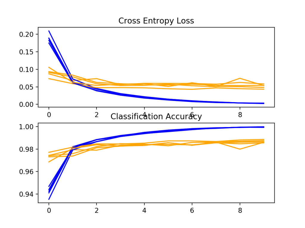 基线模型在k重交叉验证过程中的损失和精度学习曲线
接下来,计算模型性能的汇总。
我们可以看到,在这种情况下,模型的估计技巧在98.6%左右,这是合理的。
Accuracy: mean=98.677 std=0.107, n=5
最后,创建了一个箱线图来总结准确率得分的分布情况。
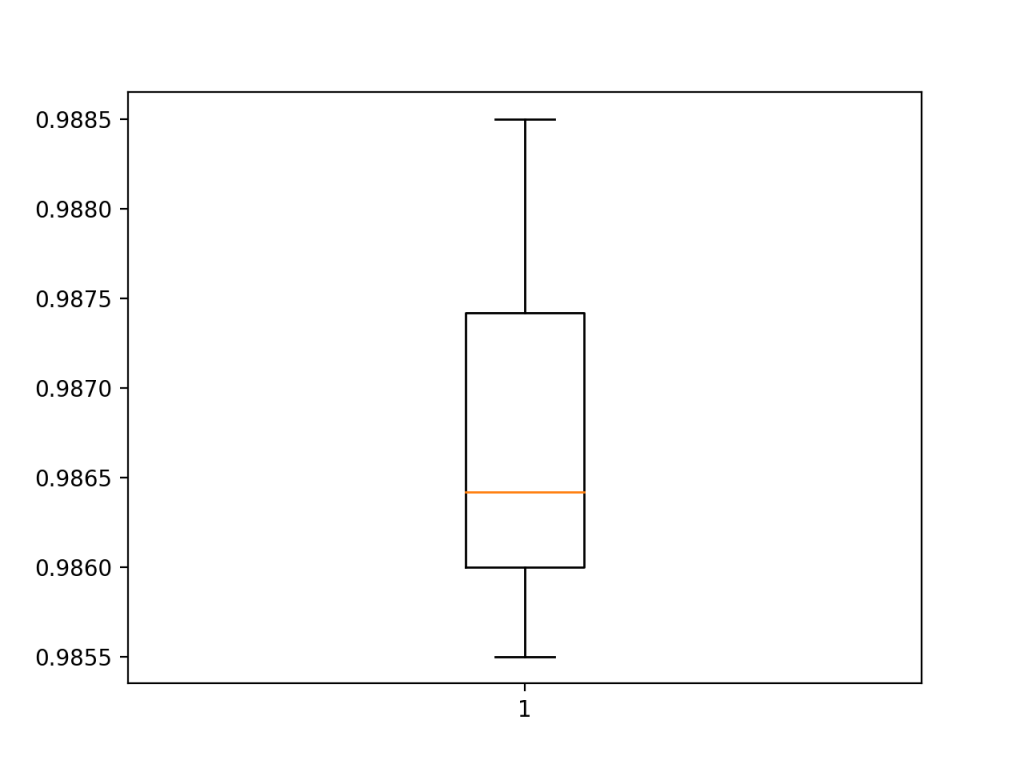 使用k倍交叉验证评估基线模型的准确度得分的箱线图
我们现在有了健壮的测试工具和性能良好的基线模型。
如何开发一种改进的模型
有很多方法可以让我们探索基线模型的改进。
我们将研究通常会带来改进的模型配置领域,即所谓的容易摘到的果实。第一个是学习算法的改变,第二个是模型深度的增加。
提高学习质量
学习算法有很多方面可以改进。
也许最大的杠杆点是学习率,例如评估学习率的较小或较大值可能产生的影响,以及在培训期间改变学习率的时间表。
另一种可以快速加速模型学习并能带来较大性能改进的方法是批处理标准化。我们将评估批处理标准化对我们的基线模型的影响。
批量归一化可以在卷积和完全连接的层之后使用。它具有改变层的输出分布的效果,特别是通过标准化输出。这有稳定和加快学习过程的效果。
我们可以更新模型定义,以便在激活函数之后对基线模型的卷积和密集层使用批归一化。下面列出了带批规范化的Define_model()函数的更新版本。
# define cnn model
def define_model():
	model = Sequential()
	model.add(Conv2D(32, (3, 3), activation='relu', kernel_initializer='he_uniform', input_shape=(28, 28, 1)))
	model.add(BatchNormalization())
	model.add(MaxPooling2D((2, 2)))
	model.add(Flatten())
	model.add(Dense(100, activation='relu', kernel_initializer='he_uniform'))
	model.add(BatchNormalization())
	model.add(Dense(10, activation='softmax'))
	# compile model
	opt = SGD(lr=0.01, momentum=0.9)
	model.compile(optimizer=opt, loss='categorical_crossentropy', metrics=['accuracy'])
	return model
下面提供了此更改的完整代码清单。
# cnn model with batch normalization for mnist
from numpy import mean
from numpy import std
from matplotlib import pyplot
from sklearn.model_selection import KFold
from keras.datasets import mnist
from keras.utils import to_categorical
from keras.models import Sequential
from keras.layers import Conv2D
from keras.layers import MaxPooling2D
from keras.layers import Dense
from keras.layers import Flatten
from keras.optimizers import SGD
from keras.layers import BatchNormalization

# load train and test dataset
def load_dataset():
	# load dataset
	(trainX, trainY), (testX, testY) = mnist.load_data()
	# reshape dataset to have a single channel
	trainX = trainX.reshape((trainX.shape[0], 28, 28, 1))
	testX = testX.reshape((testX.shape[0], 28, 28, 1))
	# one hot encode target values
	trainY = to_categorical(trainY)
	testY = to_categorical(testY)
	return trainX, trainY, testX, testY

# scale pixels
def prep_pixels(train, test):
	# convert from integers to floats
	train_norm = train.astype('float32')
	test_norm = test.astype('float32')
	# normalize to range 0-1
	train_norm = train_norm / 255.0
	test_norm = test_norm / 255.0
	# return normalized images
	return train_norm, test_norm

# define cnn model
def define_model():
	model = Sequential()
	model.add(Conv2D(32, (3, 3), activation='relu', kernel_initializer='he_uniform', input_shape=(28, 28, 1)))
	model.add(BatchNormalization())
	model.add(MaxPooling2D((2, 2)))
	model.add(Flatten())
	model.add(Dense(100, activation='relu', kernel_initializer='he_uniform'))
	model.add(BatchNormalization())
	model.add(Dense(10, activation='softmax'))
	# compile model
	opt = SGD(lr=0.01, momentum=0.9)
	model.compile(optimizer=opt, loss='categorical_crossentropy', metrics=['accuracy'])
	return model

# evaluate a model using k-fold cross-validation
def evaluate_model(dataX, dataY, n_folds=5):
	scores, histories = list(), list()
	# prepare cross validation
	kfold = KFold(n_folds, shuffle=True, random_state=1)
	# enumerate splits
	for train_ix, test_ix in kfold.split(dataX):
		# define model
		model = define_model()
		# select rows for train and test
		trainX, trainY, testX, testY = dataX[train_ix], dataY[train_ix], dataX[test_ix], dataY[test_ix]
		# fit model
		history = model.fit(trainX, trainY, epochs=10, batch_size=32, validation_data=(testX, testY), verbose=0)
		# evaluate model
		_, acc = model.evaluate(testX, testY, verbose=0)
		print('> %.3f' % (acc * 100.0))
		# stores scores
		scores.append(acc)
		histories.append(history)
	return scores, histories

# plot diagnostic learning curves
def summarize_diagnostics(histories):
	for i in range(len(histories)):
		# plot loss
		pyplot.subplot(2, 1, 1)
		pyplot.title('Cross Entropy Loss')
		pyplot.plot(histories[i].history['loss'], color='blue', label='train')
		pyplot.plot(histories[i].history['val_loss'], color='orange', label='test')
		# plot accuracy
		pyplot.subplot(2, 1, 2)
		pyplot.title('Classification Accuracy')
		pyplot.plot(histories[i].history['accuracy'], color='blue', label='train')
		pyplot.plot(histories[i].history['val_accuracy'], color='orange', label='test')
	pyplot.show()

# summarize model performance
def summarize_performance(scores):
	# print summary
	print('Accuracy: mean=%.3f std=%.3f, n=%d' % (mean(scores)*100, std(scores)*100, len(scores)))
	# box and whisker plots of results
	pyplot.boxplot(scores)
	pyplot.show()

# run the test harness for evaluating a model
def run_test_harness():
	# load dataset
	trainX, trainY, testX, testY = load_dataset()
	# prepare pixel data
	trainX, testX = prep_pixels(trainX, testX)
	# evaluate model
	scores, histories = evaluate_model(trainX, trainY)
	# learning curves
	summarize_diagnostics(histories)
	# summarize estimated performance
	summarize_performance(scores)

# entry point, run the test harness
run_test_harness()
再次运行该示例将报告交叉验证过程的每个折叠的模型性能。
我们可以看到,与交叉验证折叠中的基线相比,模型性能可能略有下降。
> 98.475
> 98.608
> 98.683
> 98.783
> 98.667
接下来,将显示一个诊断图,让你深入了解模型在每个折叠中的学习行为。
在这种情况下,我们可以看到模型总体上达到了很好的拟合,训练和测试学习曲线收敛。没有明显的过度或不适应的迹象。
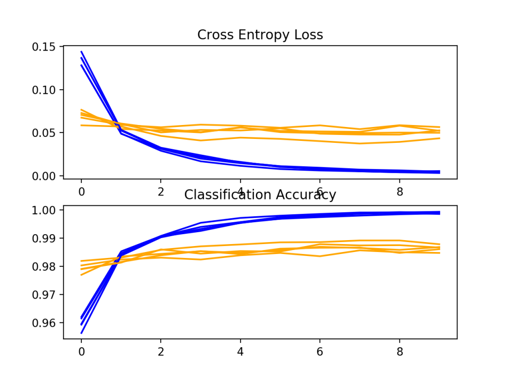 批次归一化模型在k重交叉验证过程中的损失和精度学习曲线
接下来,给出了模型的估计性能,显示了模型的平均精度略有下降的性能:98.643,而基线模型的平均精度为98.677。
Accuracy: mean=98.643 std=0.101, n=5
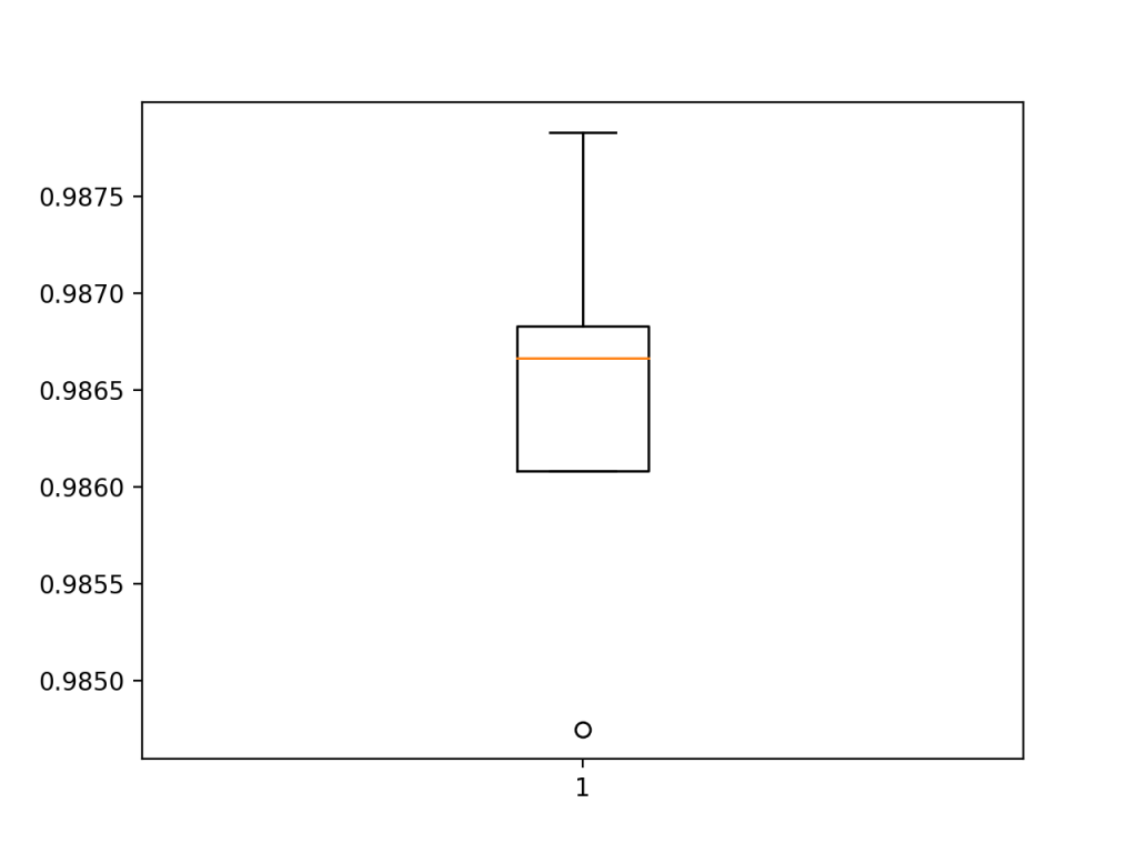 用k重交叉验证评估BatchNormalization模型准确度得分的箱线图
增加模型深度
有许多方法可以更改模型配置,以探索对基线模型的改进。
两种常见的方法包括改变模型的特征提取部分的容量或改变模型的分类器部分的容量或功能。也许影响最大的一点是特征提取器的改变。
我们可以增加模型的特征提取器部分的深度,遵循类似VGG的模式,即在增加滤波器数量的同时添加更多具有相同大小的滤波器的卷积和池化层。在这种情况下,我们将添加一个双卷积层,每个层有64个过滤器,然后是另一个最大池层。
下面列出了具有此更改的 define_model()函数的更新版本。
# define cnn model
def define_model():
	model = Sequential()
	model.add(Conv2D(32, (3, 3), activation='relu', kernel_initializer='he_uniform', input_shape=(28, 28, 1)))
	model.add(MaxPooling2D((2, 2)))
	model.add(Conv2D(64, (3, 3), activation='relu', kernel_initializer='he_uniform'))
	model.add(Conv2D(64, (3, 3), activation='relu', kernel_initializer='he_uniform'))
	model.add(MaxPooling2D((2, 2)))
	model.add(Flatten())
	model.add(Dense(100, activation='relu', kernel_initializer='he_uniform'))
	model.add(Dense(10, activation='softmax'))
	# compile model
	opt = SGD(lr=0.01, momentum=0.9)
	model.compile(optimizer=opt, loss='categorical_crossentropy', metrics=['accuracy'])
	return model
为完整起见,下面提供了包括此更改在内的整个代码清单。
# deeper cnn model for mnist
from numpy import mean
from numpy import std
from matplotlib import pyplot
from sklearn.model_selection import KFold
from keras.datasets import mnist
from keras.utils import to_categorical
from keras.models import Sequential
from keras.layers import Conv2D
from keras.layers import MaxPooling2D
from keras.layers import Dense
from keras.layers import Flatten
from keras.optimizers import SGD

# load train and test dataset
def load_dataset():
	# load dataset
	(trainX, trainY), (testX, testY) = mnist.load_data()
	# reshape dataset to have a single channel
	trainX = trainX.reshape((trainX.shape[0], 28, 28, 1))
	testX = testX.reshape((testX.shape[0], 28, 28, 1))
	# one hot encode target values
	trainY = to_categorical(trainY)
	testY = to_categorical(testY)
	return trainX, trainY, testX, testY

# scale pixels
def prep_pixels(train, test):
	# convert from integers to floats
	train_norm = train.astype('float32')
	test_norm = test.astype('float32')
	# normalize to range 0-1
	train_norm = train_norm / 255.0
	test_norm = test_norm / 255.0
	# return normalized images
	return train_norm, test_norm

# define cnn model
def define_model():
	model = Sequential()
	model.add(Conv2D(32, (3, 3), activation='relu', kernel_initializer='he_uniform', input_shape=(28, 28, 1)))
	model.add(MaxPooling2D((2, 2)))
	model.add(Conv2D(64, (3, 3), activation='relu', kernel_initializer='he_uniform'))
	model.add(Conv2D(64, (3, 3), activation='relu', kernel_initializer='he_uniform'))
	model.add(MaxPooling2D((2, 2)))
	model.add(Flatten())
	model.add(Dense(100, activation='relu', kernel_initializer='he_uniform'))
	model.add(Dense(10, activation='softmax'))
	# compile model
	opt = SGD(lr=0.01, momentum=0.9)
	model.compile(optimizer=opt, loss='categorical_crossentropy', metrics=['accuracy'])
	return model

# evaluate a model using k-fold cross-validation
def evaluate_model(dataX, dataY, n_folds=5):
	scores, histories = list(), list()
	# prepare cross validation
	kfold = KFold(n_folds, shuffle=True, random_state=1)
	# enumerate splits
	for train_ix, test_ix in kfold.split(dataX):
		# define model
		model = define_model()
		# select rows for train and test
		trainX, trainY, testX, testY = dataX[train_ix], dataY[train_ix], dataX[test_ix], dataY[test_ix]
		# fit model
		history = model.fit(trainX, trainY, epochs=10, batch_size=32, validation_data=(testX, testY), verbose=0)
		# evaluate model
		_, acc = model.evaluate(testX, testY, verbose=0)
		print('> %.3f' % (acc * 100.0))
		# stores scores
		scores.append(acc)
		histories.append(history)
	return scores, histories

# plot diagnostic learning curves
def summarize_diagnostics(histories):
	for i in range(len(histories)):
		# plot loss
		pyplot.subplot(2, 1, 1)
		pyplot.title('Cross Entropy Loss')
		pyplot.plot(histories[i].history['loss'], color='blue', label='train')
		pyplot.plot(histories[i].history['val_loss'], color='orange', label='test')
		# plot accuracy
		pyplot.subplot(2, 1, 2)
		pyplot.title('Classification Accuracy')
		pyplot.plot(histories[i].history['accuracy'], color='blue', label='train')
		pyplot.plot(histories[i].history['val_accuracy'], color='orange', label='test')
	pyplot.show()

# summarize model performance
def summarize_performance(scores):
	# print summary
	print('Accuracy: mean=%.3f std=%.3f, n=%d' % (mean(scores)*100, std(scores)*100, len(scores)))
	# box and whisker plots of results
	pyplot.boxplot(scores)
	pyplot.show()

# run the test harness for evaluating a model
def run_test_harness():
	# load dataset
	trainX, trainY, testX, testY = load_dataset()
	# prepare pixel data
	trainX, testX = prep_pixels(trainX, testX)
	# evaluate model
	scores, histories = evaluate_model(trainX, trainY)
	# learning curves
	summarize_diagnostics(histories)
	# summarize estimated performance
	summarize_performance(scores)

# entry point, run the test harness
run_test_harness()
运行示例报告交叉验证过程的每个折叠的模型性能。
每倍的分数可能表明比基线有所改善。
> 99.058
> 99.042
> 98.883
> 99.192
> 99.133
学习曲线的曲线图被创建,在这种情况下,显示模型在问题上仍然有很好的拟合,没有明显的过度拟合的迹象。这些情节甚至可能表明,进一步的训练时期可能会有所帮助。
接下来,给出了模型的估计性能,与基线相比,性能略有提高(从98.677到99.062),标准偏差也略有下降。
Accuracy: mean=99.062 std=0.104, n=5
如何最终确定模型并做出预测
只要我们有想法,并有时间和资源来测试它们,模型改进的过程就可能会持续下去。
在某种程度上,必须选择并采用最终的型号配置。在这种情况下,我们将选择更深的模型作为我们的最终模型。
首先,我们将最终确定我们的模型,但是要在整个训练数据集上拟合一个模型,并将该模型保存到文件中以备以后使用。然后,我们将加载模型并在坚持测试数据集上评估其性能,以了解所选模型在实践中的实际执行情况。最后,我们将使用保存的模型对单个图像进行预测。
保存最终模型
最终模型通常适用于所有可用的数据,例如所有训练和测试数据集的组合。
在本教程中,我们有意保留一个测试数据集,以便我们可以评估最终模型的性能,这在实践中可能是个好主意。因此,我们将仅在训练数据集上适合我们的模型。
# fit model
model.fit(trainX, trainY, epochs=10, batch_size=32, verbose=0)
一旦合适,我们就可以通过调用模型上的save()函数将最终模型保存到H5文件中,并传入所选的文件名。
# save model
model.save('final_model.h5')
注意,保存和加载Keras模型需要在你的工作站上安装h5py库。
下面列出了在训练数据集上拟合最终深度模型并将其保存到文件的完整示例。
# save the final model to file
from keras.datasets import mnist
from keras.utils import to_categorical
from keras.models import Sequential
from keras.layers import Conv2D
from keras.layers import MaxPooling2D
from keras.layers import Dense
from keras.layers import Flatten
from keras.optimizers import SGD

# load train and test dataset
def load_dataset():
	# load dataset
	(trainX, trainY), (testX, testY) = mnist.load_data()
	# reshape dataset to have a single channel
	trainX = trainX.reshape((trainX.shape[0], 28, 28, 1))
	testX = testX.reshape((testX.shape[0], 28, 28, 1))
	# one hot encode target values
	trainY = to_categorical(trainY)
	testY = to_categorical(testY)
	return trainX, trainY, testX, testY

# scale pixels
def prep_pixels(train, test):
	# convert from integers to floats
	train_norm = train.astype('float32')
	test_norm = test.astype('float32')
	# normalize to range 0-1
	train_norm = train_norm / 255.0
	test_norm = test_norm / 255.0
	# return normalized images
	return train_norm, test_norm

# define cnn model
def define_model():
	model = Sequential()
	model.add(Conv2D(32, (3, 3), activation='relu', kernel_initializer='he_uniform', input_shape=(28, 28, 1)))
	model.add(MaxPooling2D((2, 2)))
	model.add(Conv2D(64, (3, 3), activation='relu', kernel_initializer='he_uniform'))
	model.add(Conv2D(64, (3, 3), activation='relu', kernel_initializer='he_uniform'))
	model.add(MaxPooling2D((2, 2)))
	model.add(Flatten())
	model.add(Dense(100, activation='relu', kernel_initializer='he_uniform'))
	model.add(Dense(10, activation='softmax'))
	# compile model
	opt = SGD(lr=0.01, momentum=0.9)
	model.compile(optimizer=opt, loss='categorical_crossentropy', metrics=['accuracy'])
	return model

# run the test harness for evaluating a model
def run_test_harness():
	# load dataset
	trainX, trainY, testX, testY = load_dataset()
	# prepare pixel data
	trainX, testX = prep_pixels(trainX, testX)
	# define model
	model = define_model()
	# fit model
	model.fit(trainX, trainY, epochs=10, batch_size=32, verbose=0)
	# save model
	model.save('final_model.h5')

# entry point, run the test harness
run_test_harness()
运行此示例后,你现在的当前工作目录中将有一个名为‘finalModel.h5’的1.2MB文件。
评估最终模型
现在,我们可以加载最终模型,并在坚持测试数据集上对其进行评估。
如果我们对向项目涉众展示所选模型的性能感兴趣,我们可能会这样做。
模型可以通过load_model()函数加载。
下面列出了加载保存的模型并在测试数据集上评估它的完整示例。
# evaluate the deep model on the test dataset
from keras.datasets import mnist
from keras.models import load_model
from keras.utils import to_categorical

# load train and test dataset
def load_dataset():
	# load dataset
	(trainX, trainY), (testX, testY) = mnist.load_data()
	# reshape dataset to have a single channel
	trainX = trainX.reshape((trainX.shape[0], 28, 28, 1))
	testX = testX.reshape((testX.shape[0], 28, 28, 1))
	# one hot encode target values
	trainY = to_categorical(trainY)
	testY = to_categorical(testY)
	return trainX, trainY, testX, testY

# scale pixels
def prep_pixels(train, test):
	# convert from integers to floats
	train_norm = train.astype('float32')
	test_norm = test.astype('float32')
	# normalize to range 0-1
	train_norm = train_norm / 255.0
	test_norm = test_norm / 255.0
	# return normalized images
	return train_norm, test_norm

# run the test harness for evaluating a model
def run_test_harness():
	# load dataset
	trainX, trainY, testX, testY = load_dataset()
	# prepare pixel data
	trainX, testX = prep_pixels(trainX, testX)
	# load model
	model = load_model('final_model.h5')
	# evaluate model on test dataset
	_, acc = model.evaluate(testX, testY, verbose=0)
	print('> %.3f' % (acc * 100.0))

# entry point, run the test harness
run_test_harness()
运行该示例将加载保存的模型,并在坚持测试数据集中评估该模型。
计算并打印测试数据集上模型的分类精度。在这种情况下,我们可以看到,该模型达到了99.090%的准确率,或者说略低于1%,这一点也不差,相当接近估计的99.753%,标准偏差约为0.5%(例如,99%的分数)。
> 99.090
做出预测
我们可以使用保存的模型对新图像进行预测。
该模型假设新图像是灰度的,它们已经对齐,使得一个图像包含一个居中的手写数字,并且图像的大小是28×28像素的正方形。
下面是从MNIST测试数据集中提取的图像。你可以将其保存在当前工作目录中,文件名为‘sample_image.png’。
我们将假设这是一个全新的、看不见的图像,以所需的方式准备,并查看如何使用保存的模型来预测图像表示的整数(例如,我们预期为“7”)。
首先,我们可以加载图像,强制其为灰度格式,并强制大小为28×28像素。然后可以调整加载图像的大小,使其具有单个通道并表示数据集中的单个样本。load_image()函数实现了这一点,并将返回加载的图像,为分类做好准备。
重要的是,像素值的准备方式与在拟合最终模型时为训练数据集准备像素值的方式相同,在这种情况下,是归一化的。
# load and prepare the image
def load_image(filename):
	# load the image
	img = load_img(filename, grayscale=True, target_size=(28, 28))
	# convert to array
	img = img_to_array(img)
	# reshape into a single sample with 1 channel
	img = img.reshape(1, 28, 28, 1)
	# prepare pixel data
	img = img.astype('float32')
	img = img / 255.0
	return img
接下来,我们可以像上一节那样加载模型,并调用predict_classes()函数来预测图像表示的数字。
# predict the class
digit = model.predict_classes(img)
下面列出了完整的示例。
# make a prediction for a new image.
from keras.preprocessing.image import load_img
from keras.preprocessing.image import img_to_array
from keras.models import load_model

# load and prepare the image
def load_image(filename):
	# load the image
	img = load_img(filename, grayscale=True, target_size=(28, 28))
	# convert to array
	img = img_to_array(img)
	# reshape into a single sample with 1 channel
	img = img.reshape(1, 28, 28, 1)
	# prepare pixel data
	img = img.astype('float32')
	img = img / 255.0
	return img

# load an image and predict the class
def run_example():
	# load the image
	img = load_image('sample_image.png')
	# load model
	model = load_model('final_model.h5')
	# predict the class
	digit = model.predict_classes(img)
	print(digit[0])

# entry point, run the example
run_example()
运行该示例首先加载并准备图像,加载模型,然后正确预测加载的图像表示数字“7”。
7
拓展
本节列出了一些你可能希望了解的扩展教程的想法。
- 调整像素缩放。探索与基线模型相比,替代像素缩放方法如何影响模型性能,包括居中和标准化。
- 调整学习速率。了解与基准模型(例如0.001和0.0001)相比,不同的学习速率对模型性能有何影响。
- 调整模型深度。探索与基线模型相比,向模型添加更多层对模型性能有何影响,例如模型的分类器部分中的另一块卷积和池层或另一个致密层。
进一步阅读
如果你想深入了解,本节提供了更多关于该主题的资源。
APIs
文章
摘要
在本教程中,你了解了如何从头开始开发用于手写数字分类的卷积神经网络。
具体地说,你了解到:
- 如何开发测试工具来开发模型的健壮评估,并为分类任务建立性能基线。
- 如何探索基线模型的扩展以提高学习和建模能力。
- 如何开发最终的模型,评估最终模型的性能,并使用它对新图像进行预测。

